목차
Density Estimation이란,,
$\;\;$Density Estimation 이란, observation 데이터셋 $x_1, \cdots, x_N$가 주어졌을 때, random variable $x$의 probability distribution $p(x)$를 찾는 것(modeling) 입니다. 이때, 각각의 데이터는 I.I.D(independent and identically distributed)를 가정하고 있습니다.
Parametric estimation vs Nonparametric estimation
$\;\;$Density Estimation에는 크게 2가지 접근이 가능합니다.
$\rightarrow$ Parametric estimation & Nonparametric estimation
첫째, Parametric estimation 은 관찰한 데이터셋에 적합한 특정 함수가 있다고 가정하고, 함수를 이루는 parameters를 찾습니다. 만약 특정 함수를 Gaussian으로 가정했다면, $u, \sigma^2$을 찾아야 합니다. 구체적인 함수를 찾았다면, 새로운 데이터에 대해서 추론(infer)하기 쉽습니다. 하지만 데이터가 찾은 함수에 딱 들어맞지 않을 수도 있다는 단점이 있습니다.
둘째, Nonparametric estimation 은 특정 함수를 가정하지 않습니다. 대신, 온전히 관찰한 데이터에 기반하여 probability distribution을 찾습니다. 데이터에 대한 가정 없이 estimation을 수행하기 때문에 관찰한 데이터에 들어맞는 distribution을 찾기 쉽습니다. 하지만, 새로운 데이터가 추가되면 분포가 달라진다는 단점이 있습니다. Kernel function은 대표적인 nonparametric estimation입니다. $f(x) = \frac{1}{N}\sum^N_{i=1}K_h(x-x_i)$
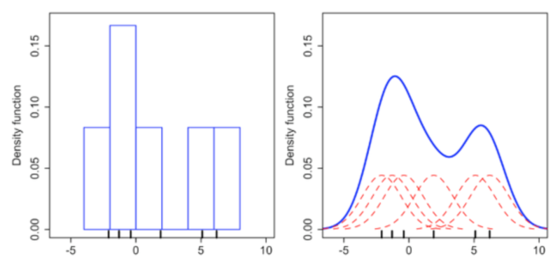
추가적으로, 두 접근의 장점을 합친 Semi-parametric estimation도 존재합니다. mixture model, feedforward neural net이 여기에 해당합니다.
본 포스팅에서는 parametric estimation에 집중합니다!!
parametric estimation 문제를 풀기 위해서는 3가지 방법, (1) MLE, (2) MAP, (3) Bayesian Inference이 있습니다.
MLE, MAP vs Bayesian Inference
(1) MLE와 (2) MAP는 frequentist treatment이고, 특정한 criterion(e.g. likelihood function)을 최적으로 만족하는 구체적인 parameter를 찾습니다. 반면, (3) Bayesian Inference는 prior distribution을 이용해 Bayes이론을 적용하여 posterior distribution을 구합니다.
매우매우 직관적으로 비교해보면, MLE와 MAP는 데이터를 가장 잘 설명하는 단 한쌍의 parameter $\lambda_*, \gamma_*$를 찾습니다. 그리고 새로운 데이터에 대해 예측할 때 최적의 parameter 모델($\theta_*$)을 통해 probability prediction을 구합니다.$$\rightarrow p(x|\theta_*)$$
반면, Bayesian inference는 여러 모델(여러 쌍의 parameter)가 데이터를 설명할 것이라고 가정합니다. 예를 들면 다섯 쌍의 $\lambda, \gamma$를 찾습니다. 이를 통해 동일한 prior를 갖는 5개의 posterior 모델이 생성됩니다. 새로운 데이터 예측 시, 5개 모델의 결과를 weighted sum(weight : $p(\theta_i|D)$)하여 최종 예측 결과를 구하게 됩니다. $$\rightarrow \sum_{i=1}^5 p(x|\theta_i) p(\theta_i|D)$$
왜 Gaussian Distribution인가? $\rightarrow$ 포스팅 추가
1. Maximum Likelihood Estimation (MLE)
MLE는 말 그대로 likelihood function 를 최대로 하는 parameter을 구하는 방법입니다.
데이터 셋 $X = {x_1, \cdots, x_n}$에서 각 데이터가 $p(x|\theta)$분포에서 독립졌으로 뽑혔다고 가정할 때, likelihood function은 다음과 같습니다. $$p(X|\theta) = \prod^N_{t=1}p(x_t|\theta)$$
자 이제 여기서 미분을 취해서 최대값을 찾는 것이 보통인데, 식이 곱으로 연결되어있기 때문에 미분이 어렵습니다. 따라서 log를 취해주면서 곱 $\rightarrow$ 합 으로 풀어줍니다. log는 단조증가함수이기 때문에 likelihood function과 log를 취한 log likelihood function의 최대값이 같습니다.
log-likelihood :
$$L(\theta) = \sum^N_{t=1}p(x_t|\theta)$$
ML의 목표는 log-likelihood 최대화 하는 parameter 찾기! $\hat{\theta_{ML}} = \arg\max_\theta L(\theta)$ 입니다.
최적의 parameter값 $\theta_{ML}$을 구했다면 $p(x_*|\theta_{ML})$을 통해 prediction 문제를 풀면 됩니다.
왜 MLE가 잘 작동할까요?? Kullback Matching 관점에서 살펴봅시다~~
우선, Empirical distribution은 주어진 데이터들이 각각 동일한 $\frac{1}{N}$의 확률을 가지는 분포입니다.
Empirical distribuion : $\textcolor{green}{\tilde p(x) = \frac{1}{N}\sum_{t=1}^N \delta(x-x_t)}$
예측 모델을 통해 sample한 데이터셋이 empirical distribution에서 sample한 데이터셋과 유사해야 모델이 데이터를 잘 표현한다고 할 수 있습니다. 즉, 모델 $\textcolor{red}{p(x|\theta)}$과 Empirical distribution과 닮아져야 합니다. 이를 위해서, 두 확률 분포의 차이를 계산하는 함수인 Kullback–Leibler divergence(KLD)를 사용합니다. KLD는 어떤 이상적인 분포($\textcolor{red}{\rightarrow \tilde p(x)}$)에 대해, 그 분포를 근사하는 다른 분포($\textcolor{green}{\rightarrow p(x|\theta)}$)를 사용했을 경우 발생할 수 있는 정보의 양, entropy 차이를 계산합니다. 따라서 차이를 최소화하는, $\arg\min_\theta KL[\textcolor{red}{\tilde p(x)}|\textcolor{green}{p(x|\theta)}]$ 를 만족하는 $\theta$를 찾아야 합니다. $$\begin{align*}\arg\min_\theta KL[\tilde p(x)|p(x|\theta)]=\arg\min_\theta \int \textcolor{red}{\tilde p(x) \log} \frac{\textcolor{red}{\tilde p(x)}}{p(x|\theta)}dx\\=\arg\min_\theta[ \textcolor{red}{-H(\tilde{p}}) -\int \tilde p(x) \log p(x|\theta)dx]\end{align*}$$
이때, $\tilde{p}$의 entropy에 해당하는 $\textcolor{red}{-H(\tilde{p})}$는 $\theta$를 구하는데 관련이 없기 때문에, 다음과 같이 정리됩니다.
$$\begin{align*}\arg\max_\theta E_{\tilde{p}} \log p(x|\theta) = \arg\max_\theta \frac{1}{N} \int \sum_{t=1}^N \delta(x-x_t) \log p(x|\theta)dx\\=\arg\max_\theta \frac{1}{N}\sum_{t=1}^N \log p(x_t|\theta)\end{align*}$$
$\arg\max_\theta \frac{1}{N}\sum_{t=1}^N \log p(x_t|\theta)$ 는 앞서 구한 MLE 방법에서의 $\theta$와 일치하는 것을 확인할 수 있습니다.
추가적으로 관측되지 않았지만 모형의 해석을 돕기 위해 latent variable $s$를 도입하면, 모델은 $p(x|\theta) = \int p(x,s|\theta)ds$ 이고, MLE를 통해 $\arg\max_\theta \log \int p(x,s|\theta)ds$인 $\theta$를 찾습니다. 이 경우에는 EM 알고리즘을 적용하여 해결합니다. :) (자세한 내용은 4장에서 다룹니다!) EM설명: https://zephyrus1111.tistory.com/89
Univariate Normal 의 예시로 MLE를 살펴봅시다.
$$p(x|\theta) = \frac{1}{\sqrt{2\pi}\sigma}exp\{-\frac{1}{2\sigma^2}(x-u)^2\}$$
이때 구해야하는 target $\theta$는 $\theta_1=u, \theta_2 = \sigma^2$ 입니다.
STEP 1) log-likelihood $L(\theta)$를 구합니다.
$$\begin{align*}L(\theta) = \sum_{t=1}^N \log p(x_t|\theta) \\ = \sum_{t=1}^N[-\frac{1}{2}\log 2\pi \theta_2 - \frac{1}{2\theta_2}(x_t-\theta_1)^2]\end{align*}$$
STEP 2) log-likelihood에 미분을 취하여 $\nabla_\theta L(\theta)$ 를 구합니다.
우선, $\theta_1$인 $u$에 대해 편미분 해봅시다.
$$\frac{\partial L(\theta)}{\partial u} = \frac{1}{\sigma^2} \sum_{t=1}^N(x_t-u)$$
다음으로 $\theta_2$인 $\sigma^2$에 대해 편미분 해봅시다.
$$\frac{\partial L(\theta)}{\partial \sigma^2} = -\frac{N}{2\sigma^2} -\frac{1}{2}\sum_{t=1}^N(x_t-u)^2(\frac{-1}{(\sigma^2)^2})$$
STEP 3) $\nabla_\theta L(\theta) = 0$ 으로 설정하고, $u, \sigma^2$를 구합니다.
STEP 2 에서 구한 2개의 편미분 식을 각각 0으로 설정하고 풀어보면 다음과 같이 구할 수 있습니다. $$u = \frac{1}{N}\sum_{t=1}^N x_t$,\;\;\; \sigma^2 = \frac{1}{N} \sum_{t=1}^N (x_t-u)^2$$
2. MAP
다음 방법은 Maximum a Posterior (MAP)입니다. MAP 는 말그대로 posterior을 최대화하는 parameter를 찾는 방법입니다. Bayes rule을 이용해 prior $\log p(\theta)$ 과 likelihood로 Bayesian posterior를 계산합니다. prior는 overfitting 문제를 방지할 수 있으며, 모델이 너무 복잡해지는 것을 막는 regularizer역할이기도 합니다. MLE, MAP중 어느것이 좋은지는 단정할 수 없지만 prior에 대한 정보가 있을 때는 MAP를 사용하는 것이 유리합니다. MLE는 prior probability가 uniform distribution이라고 가정한 MAP라고 볼 수 있습니다. (https://sanghyu.tistory.com/10)
https://machinelearningmastery.com/maximum-a-posteriori-estimation/
$$\tilde \theta_{MAP} = \arg\max_\theta p(\theta|x) \\ = \arg\max_\theta \frac{p(x|\theta)p(\theta)}{p(x)} \\ = \arg\max_\theta p(x|\theta)p(\theta) \\ = \arg\max_\theta [\log p(x|\theta)+ \log p(\theta)]$$
Univariate Normal 의 예시로 MAP를 살펴봅시다.
$X \sim N(u,1)$ 이고, prior $p(u) \sim N(0,\alpha^2)$ 라고 가정합시다.
STEP 1) log Posterior를 계산합니다.
$$L = \log p(X|\theta)+\log p(\theta) \\ \propto -\frac{1}{2} \sum_{t=1}^N(x_t-u)^2 -\frac{1}{2\alpha^2}u^2$$
STEP 2) u에 대해 편미분을 취합니다.
$$\frac{\partial L}{\partial u} = \sum_{t=1}^N (x_t-u)-\frac{1}{\alpha^2}u$$
STEP 3) $\frac{\partial L}{\partial u} = 0$ 으로 설정하고, $\tilde u_{MAP}$를 구합니다.
$$\tilde u_{MAP}=\frac{1}{N+\frac{1}{\alpha^2}}\sum_{t=1}^N x_t$$
이때 데이터의 수 $N\gg\frac{1}{\alpha^2}$ 이라면, prior의 영향이 무시됩니다. 이럴 경우, $\tilde u_{MAP} \rightarrow \tilde u_{ML}=\frac{1}{N}\sum_{t=1}^N x_t$ 입니다.
반면, $\frac{1}{\alpha^2}\gg N$의 경우, prior이 영향이 커집니다. 따라서 prior가 $p(u) \sim N(0,\sigma^2)$인 예시에서 $\tilde u_{MAP} \rightarrow 0$가 됩니다.
3. Bayesian Inference
Bayesian inference는 parameter $\theta$를 random variable로 설정합니다. 그리고 이 random variable에 대한 prior knowledge가 관찰된 데이터셋 D에 따라 어떻게 변하는지 찾고자 합니다.
MLE, MAP와 달리 parameter의 구체적인 값을 구하는 것이 아니라, $\theta$에 대한 모든 값의 posterior density를 찾습니다. (= determine the posterior density over all values for $\theta$)
Posterior distribution : $$p(\theta|d) = \frac{p(d|\theta)p(\theta)}{\int p(d|\theta)p(\theta) d\theta} = \frac{likelihood * prior}{marginal \; likelihood\;(or\; evidence)} $$
Bayesian inference를 통해 구한 posterior distribution을 unsupervised, supervised Bayesian에 어떻게 사용할 수 있을까요? Bayesian inference는 앞에서도 강조했듯이 구체적인 값을 구하는 것이 아니라 모든 가능한 $\theta$를 구합니다. 따라서 모든 가능한 $\theta$에 대해서 weighted averge 값을 계산하게 됩니다. (integrate over all possible values of $\theta$)
(1) unsupervised Bayesian은 데이터셋 $D$가 주어졌을때, 새로운 데이터 x의 probability를 얻는 것이 목적입니다.
$$p(x|D) = \int p(x,\theta|D)d \theta \\ =\int p(x|\theta,D)p(\theta|D)d \theta \\=\int p(x|\theta)p(\theta|D)d \theta$$
(2) supervised Bayesian은 target value y의 probability를 얻는 것이 목적입니다.
$$p(y|x,D) = \int p(y|x,\theta)p(\theta|D)d\theta$$
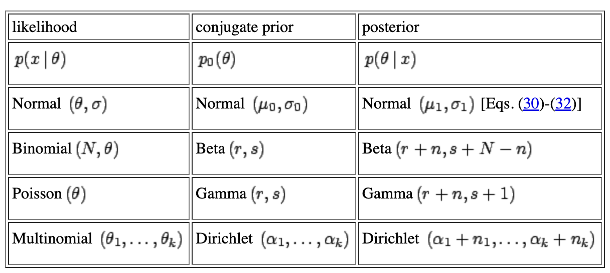
posterior 계산 시에는 conjugate prior을 사용합니다.
conjugate prior란, posterior이 prior과 같은 포맷이게 하는 prior을 의미합니다.
Bayesian Inference도 Gaussian 예제로 마무리 짓겠습니다.
$x \sim N(u,\sigma^2), \sigma^2$은 알고있다고 가정하며, prior : $u \sim N(u_0, \sigma_0^2)$
STEP 1) posterior을 계산합니다.
$$p(u|D) = \frac{p_o(u)}{p(D)\prod_{t=1}^N p(x_t|u}$$
STEP 2) 계산을 통해 posterior mean $\tilde u, posterior variance \tilde \sigma^2$를 구합니다.
$$\tilde u = (\frac{N\sigma_0^2}{N\sigma_0^2+\sigma^2})u_{ML}+\frac{\sigma_0^2}{N\sigma_0^2+\sigma^2}u_0$$
$$\tilde \sigma^2 = \frac{\sigma_0^2 \sigma^2}{N \sigma_0^2+\sigma^2}$$
데이터 수 $N=0$이면, $\tilde u$는 prior mean($u_0$) , $\tilde \sigma^2$는 prior variance가 됩니다.
데이터 수 $N\rightarrow \inf$이면, $\tilde u$는 $u_{ML}$, $\tilde \sigma^2$는 0이 됩니다. 즉 MLE의 방법과 일치하게 됩니다. (infinitely peaked around the ML solution)
아래 그림은 $x \sim N(0.8,0.1), prior mean 0일 경우, 데이터 수에 따른 여러 posterior distribution을 보여줍니다.

'ML&DL > Pattern Recognition and Machine Learning' 카테고리의 다른 글
| 6. Latent Variable Models PCA & FA & MFA (0) | 2022.11.04 |
|---|---|
| 5. Expectation Maximization(EM) (1) | 2022.10.25 |
| 4. Clustering (1) | 2022.09.22 |